When you want to format cells in Microsoft Excel, you can do it manually, by selecting fonts, font color and size, background colors and borders, or you can do the formatting quickly and automatically using styles. If you used styles in other programs, you’ll be familiar with the concept: a style is a mixture of formatting that you can apply over and over, like paint.
There are two advantages to using styles:
- Speed. When you have a lot of cells to format, it’s faster to apply a style than to apply all the formatting features individually. And if you need to change a formatting feature of all the cells – like just the color or the font – changing the style definition will immediately update the cell formatting.
- Consistency. When formatting a lot of cells, it’s easy to make a mistake and select a slightly different color or font size. But when you apply styles, the exact, same formatting gets applied every time.
Excel has built-in styles that you can use, and you can also modify them and create your own. Here's how.
Note: If you're looking to format your tables for display on the web, try the Excel to HTML converter which is no longer available on Envato Market. It converts your Excel spreadsheets to responsive, fully formatted HTML tables.
Screencast
If you want to follow along with this tutorial using your own Excel file, you can do so. Or if you prefer, download the zip file included for this tutorial, which contains a sample workbook called excel styles.xlsx.
Using Built-In Styles
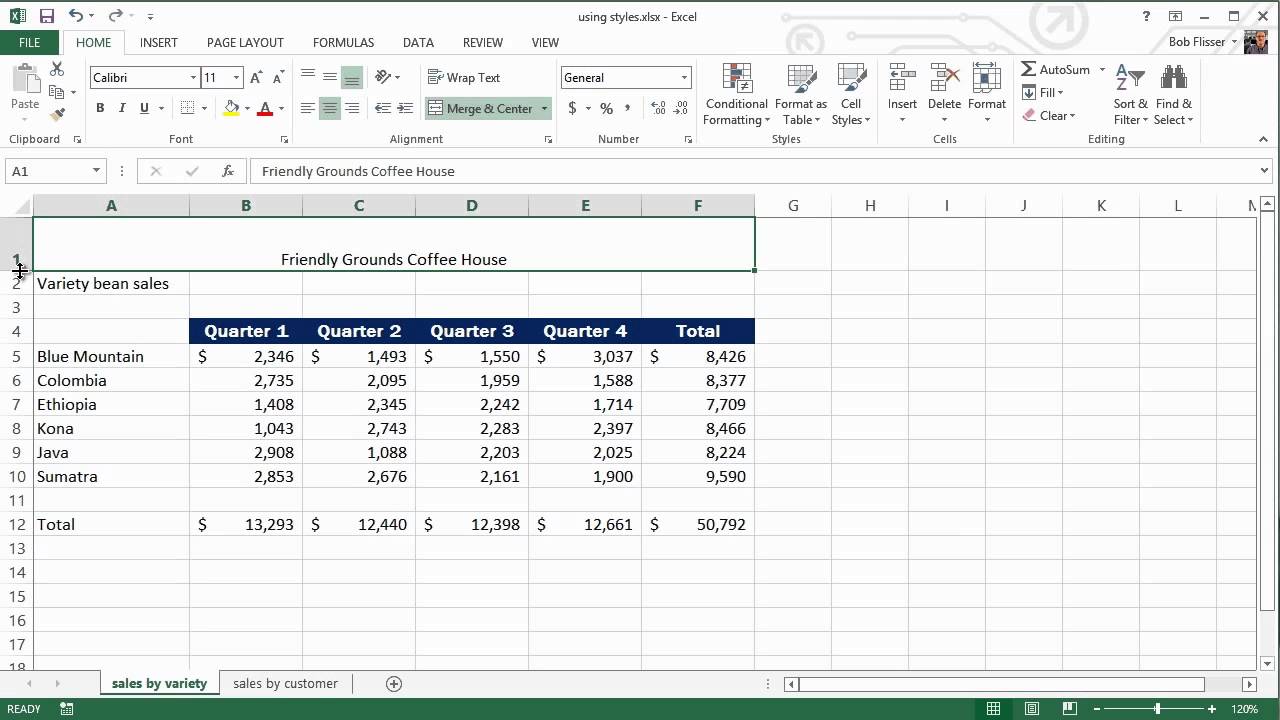
Excel has several built-in styles that you can use, so let’s start with those. First, select the row of column headers in the first worksheet of the workbook (B4:F4).


On the Home tab of the ribbon bar, you’ll find the styles on the right side. Depending on how wide your screen is, styles will either be a single button, or an area with a down arrow in the lower-right corner. Click whichever one you see (this screen capture is from the Windows version, and the Mac version is almost identical).


Roll the mouse pointer over any of the styles to see a preview of how it looks on the worksheet (Windows, only). Note: the style names, like Good, Bad, and Title, are just suggested uses. You can use any style for any purpose you want.


Click one to apply it to the selection, then click somewhere in the worksheet to deselect and get a better look.


Now go to the second worksheet (Sales by Customer) and repeat: select the column headers along row 5 and apply the same style. Deselect to get a better look


So far, it doesn't seem very impressive, but here’s where it gets cool: changing the formatting by changing the style.
Modifying a Built-In Style
Select any of the cells you just formatted, then go back to the Styles drop-down and right-click the style you just applied. Select Modify from the pop-up menu.


The dialog box that appears shows what parts of the formatting are included in the style.


So for example, you might have a style that includes fonts and color information, but doesn’t affect number formatting. Or vice-versa. For this example, we’ll change the font, color and background, and add alignment to the style.
Click the Format button at the top of the dialog, and that brings up the regular Format Cells dialog. Make the following changes:
Alignment tab: set Horizontal alignment to Center


Font tab: choose a heavier weight font and slightly larger size (I chose Franklin Gothic Medium, 12 pt.), white color


Fill tab: choose a dark color


Click OK. Notice that the Style dialog box shows that Alignment is now part of the style. Click OK again.
Not only did the column headers change in the current workbook, but when you click the tab for the first workbook, you’ll see they changed, also.


Even better, you don’t have to depend on the built-in styles. You can create your own.
Creating and Applying a Custom Style
The best way to create a custom style is to format a cell the regular, manual way, then create a style from the example formatting. We’ll do that with the worksheet titles.
But what styles cannot do is control worksheet structure, so we have to do that, first. On the first worksheet, make cell A1 twice the height, and merge cells A1:F1 (select the cells, then click Merge & Center on the Home tab of the ribbon bar).
With the merged cell selected, apply the following formats:
- Different boldfaced font (I chose Impact)
- Larger size
- Dark background color, light foreground color
- Thick box border
- Vertically centered


Click back on the Styles button or section, then select New Cell Style.


Give it a name of Sheet Title, then select all check boxes except the first one. Click OK.


Now use the style in the other worksheet. Go to the second worksheet, then as you did in the first worksheet, select and merge the top 7 cells (A1:G1) and make the row taller. Click in the Styles button or section, then select the Sheet Title style, which will be at the top of the list.


Using the Custom Style in Another Workbook
When you create styles, they’re available only in the sheets of the workbook where you created it. To use custom styles in other workbooks, you need to import them.
Open the file called Merging Styles.xlsxs, which is the other file included with this tutorial. Or you can use your own file. But don’t close the workbook you’ve been working on. It must remain open for you to get the styles.
Click the Styles button or section, and you’ll see only the default styles. Your custom style isn’t there, and the built-in style you modified has the original look. So at the bottom of the styles, click Merge Styles in Windows, or Import Cell Styles in the Mac version.


The dialog box that appears will display the other open file (you may have more than one). Double-click Using Styles.xlsx (or other file, if you used your own), then click Yes in the message box that asks you to confirm.
Now we can use the styles we just imported. Select the column headers along row 5 (A5:M5), then apply the Accent 1 style. Select and merge the top 13 cells (A1:M1), make row 1 taller, then apply the Sheet Title style.


Conclusion
Now you can see why styles are so great: it’s faster to apply a style than it is to apply multiple formatting attributes, and there isn’t any chance that cells of the same style will have different attributes because of human error. Also, when you change the look of a style, all cells formatted with that style will change immediately. And to use the styles from one workbook in another workbook, remember that they both have to be open.
Next time you need to change the style of a spreadsheet, don't change each element individually. Instead, use these tricks to format your spreadsheet with styles, and see how much time you can save by not having to change formatting for each individual column or cell.
 By
By